Jack in a Cup Simulation
Northwestern University’s ME314 Machine Dynamics class focuses on analysis of rigid body systems using Lagrangian dynamics, including how to deal with external forces, constraints, and impacts. The class also puts a heavy emphasis on using numerical methods and Python’s sympy, numpy, and plotly packages to simulate system behavior and then animate that simulation.
As a final project in the class, students model a dynamic rigid body system, simulate it, and animate it. I modeled a jack bouncing around in a cup. Both these rigid bodies are subject to gravity, and the cup is subject to two orthogonal external forces and an external torque (to mimic a human shaking it).
Here is a video of the final simulation:
Overview of Methodology
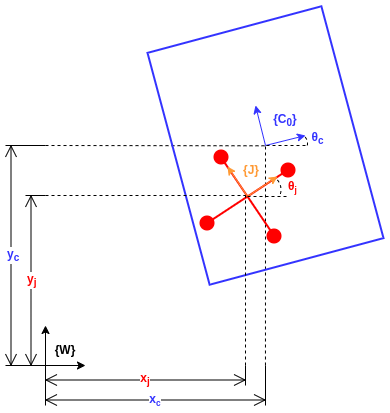
The system consists of two rigid bodies, the jack and the cup, simulated in a 2D plane. Each body has 3 degrees of freedom (orientation and 2D position), giving a total of 6 configuration variables for the system.

The system’s configuration variables.
The dynamics modeling of the system relies heavily on SE(3) transformation matrices to describe transformations between reference frames. These are used not only to construct the Lagrangian and Euler-Lagrange equations, but also to detect impact conditions and apply impact updates.


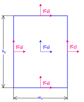
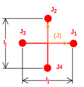
Cup and jack dimensions and frames.
All impacts are considered elastic. Because simultaneous impacts in elastic systems are underspecified, simultaneous impacts were ignored and treated as just single impacts.
For more information on the system and other modeling choices, see the project’s detailed description in the Jupyter Notebook.
The simulation follows these steps:
- Define the system state variables.
- Define frames to describe the system using the state variables.
- Define kinetic and potential energies in the system using the state variables and other system information.
- Define external forces/torques.
- Construct the system Lagrangian.
- Derive the system Euler-Lagrange equations.
- Solve the system Euler-Lagrange equations for the second derivatives of the state variables.
- Define impact conditions based on the system geometry.
- Derive impact update equations based on the impact conditions and assuming elastic impact.
- Simulate for a 5 second timespan using a timestep of 0.01 seconds.
- Calculate the state at each timestep using the solutions to the Euler-Lagrange equations and a Runge-Kutta fourth-order integration scheme.
- Check all impact conditions at each timestep. If impacts occurred, apply the appropriate impact update and resume the simulation.
- Animate simulation results.
Conclusions
The Lagrangian dynamics analysis method - especially when used in concert with SE(3) transformation matrices - gives a procedural way to analyze a system. I find this method very useful especially when systems are more complex than basic, simple systems with only a few configuration variables, as most engineering systems are. The behavior of these complex systems can be very difficult to predict, so having a procedural method of analysis helps me trust that my analysis will be correct.
On top of that, from this class I’ve learned the value of visualizing simulations, especially with animations. Solutions to the Euler-Lagrange equations can be quite messy, and are often hard to interpret just from looking at them. However, an animation provides a visual whose validity can be judged much more easily using physical intuition. Of course, other tools like analyzing conserved quantities are also critical for judging the validity of a solution.
I’ve gained an appreciation for how quickly systems can become complex. This system itself is fairly simple in the grand scheme of things - only six configuration and sixteen impact conditions between two rigid bodies. And yet finding symbolic solutions and simulating still takes a few minutes. As more rigid bodies and configuration variables are added, systems very quickly become very complex and take long amounts of time to solve. For these reasons, it’s important to be smart when defining a system, make simplifications when necessary, and pay attention to code efficiency when simulating complex systems.
Finally, I’ve learned that because systems become so complex, it’s important to understand that these simplifications and modeling choices exist in any simulation out there. For example, my choice to treat simultaneous impacts as single impacts seemed to work well enough for this system, but it might cause huge problems in another simulation. Being cognizant of these choices can be very important when analyzing simulation behavior and understanding how the simulation will differ from system behavior in the real world.