EKF SLAM from Scratch
Northwestern University’s ME495 Sensing, Navigation, and Machine Learning class is centered around one large project: implementing feature-based Extended Kalman Filter Simultaneous Localization and Mapping (SLAM) on a TurtleBot3 using C++ and ROS 2 Humble.
During this class I created several packages from scratch to accomplish this task in both simulation and with a real robot.
The video above shows this project in action. The RVIZ window on the right shows several key features:
- LiDAR point data (yellow dots)
- Robot odometry position estimate (blue robot)
- Robot EKF SLAM position estimate (green robot)
- Landmark EKF SLAM position estimate (green cylinders)
As can be seen, the EKF SLAM estimate follows the real-world position of the robot closely, even as the odometry estimate drifts.
Table of Contents
SLAM Pipeline
This project’s EKF SLAM pipeline relies on data from two sensors: encoders in the robot’s wheel motors and a 2D LiDAR on top of the robot. This data is used in conjunction with previous state estimates to estimate the current state of the robot and landmarks in a controlled environment.

The Extended Kalman Filter SLAM pipeline used for this project.
Odometry
Wheel encoder data arrives at 200 Hz, much faster than the LiDAR data at 5Hz. For this reason it can be used for state estimates in between the SLAM updates.
Odometry uses the forward kinematics of the TurtleBot3’s differential drive design to calculate the theoretical location of the robot based on how the wheels have turned, assuming no slipping occurs.
However, slipping does in fact occur, meaning that over time the odometry estimate will drift away from the real location of the robot. This can be seen in the video above.
Landmark Detection and Data Association
We’d like to improve the state estimate from odometry by looking at data from the world around us. This is where the 2D LiDAR data comes in. Our controlled environment has cylindrical obstacles in it, which can be used as landmarks for positioning the robot in the environment.
However, the LiDAR data comes in as a series of data points giving us how far away an object is (range) and the angle from the front of the robot (bearing). In order to interpret this data as “cylinders,” it’ll have to be processed a few different ways.
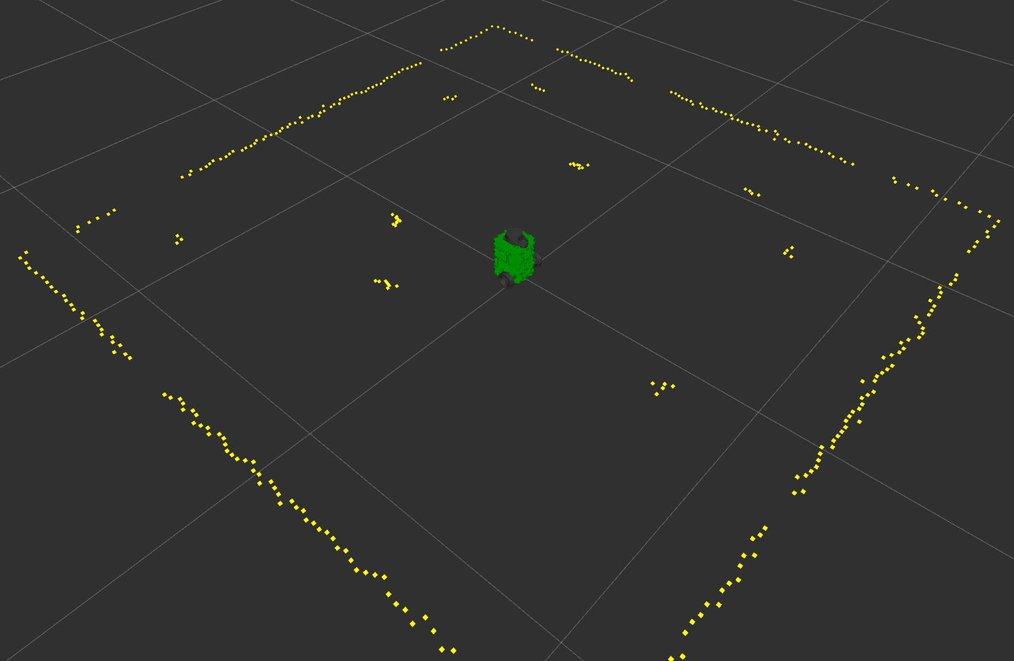
Raw LiDAR data, which won’t mean much until processed.
Point Clustering
First, a simple unsupervised DBSCAN-like learning algorithm is used to group the LiDAR points into clusters based on their Euclidean distance from each other. Each cluster is considered a possible landmark.
Circle Classification and Regression
Clusters are filtered using a circle detection algorithm to determine which are likely to represent cylindrical landmarks and which are not.
Then, a supervised learning algorithm performs Gaussian process regression to determine the best fit circle for each cluster of points. If the radius of the fit circle is too large or small (based on adjustable thresholds), a certain cluster is thrown out.
The center of the remaining circles is considered the coordinates of a detected landmark.
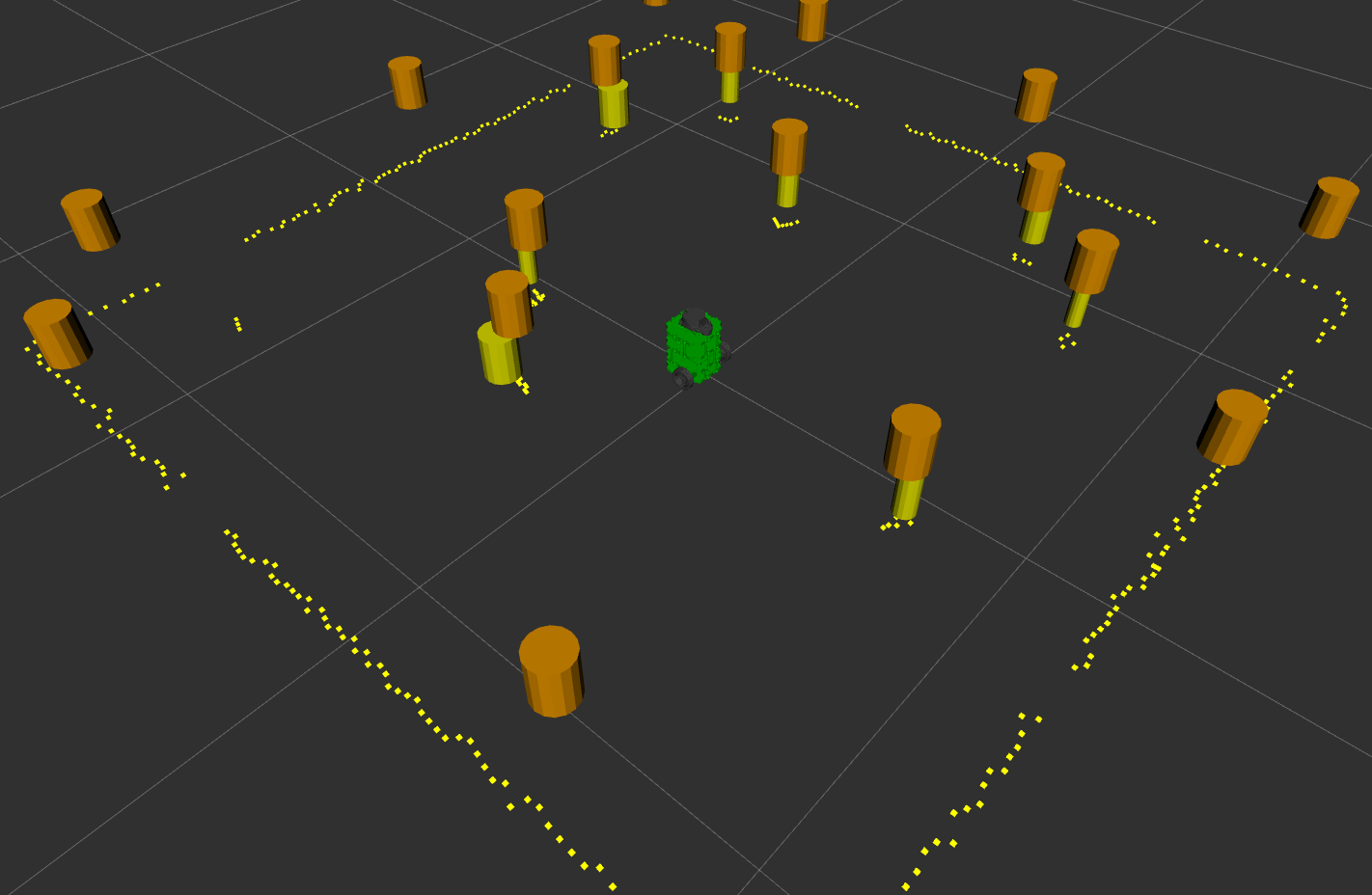
Detected clusters (orange cylinders) and detected circles (yellow cylinders).
As can be seen above, although the environment walls still appear as clusters, the circle classification/filtering successfully identifies only the actual landmarks.
Mahalanobis Distance
Finally, the detected landmarks must be associated with previously witnessed landmarks. This is done using Mahalanobis distance, which takes into account the covariance of the previous detections. If a detected landmark has a Mahalanobis distance less than a certain adjustable threshold to a previous detection, it is considered another detection of that landmark. If a landmark is above that threshold for all previous detection, it is considered a new landmark detection.
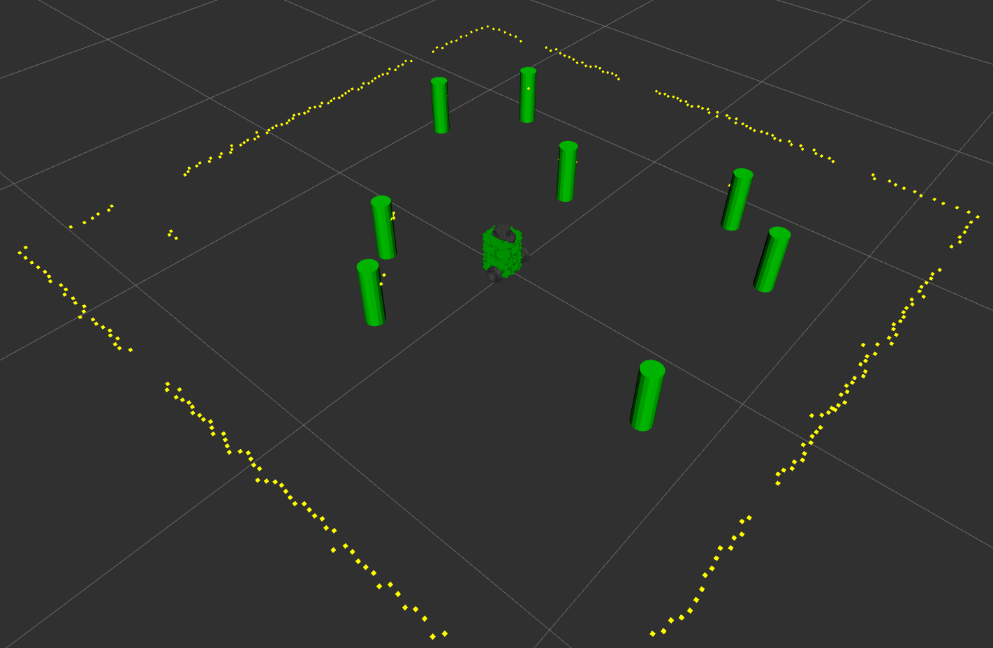
After data association, fit circles can be recognized as landmarks in the environment.
This finally allows us to transform raw 2D LiDAR into associated landmarks, which will help us position the robot during SLAM updates.
Extended Kalman Filter SLAM
Now that we have landmark data to help localize the robot within the environment, feature-based Extended Kalman Filter SLAM can be performed. There are two steps to this, prediction and correction.
Prediction
In the prediction step, the difference in odometry between the current and last SLAM updates is used to predict a new state and covariance of the robot. Because odometry inaccuracies can accumulate over time, this prediction may not be accurate.
Correction
In the correction step, the detected landmarks are used to iteratively update the predicted state. Kalman gains are calculated by taking into account the expected location of the landmark (based on the state prediction) and its actual detected location. Then the robot state and covariance are updated appropriately.
The result is a much more accurate position for the robot than can be obtained from odometry alone.
Simulation
In order to test the complex pipeline above, I wrote a simulation package. This package essentially replaces the real robot by simulating the sensor data and motion of the robot. It has adjustable parameters for simulating sensor noise and wheel slippage.
Here is a video of the EKF SLAM pipeline working in simulation.
Here’s a key for interpreting the items in the video:
- Red - the simulation’s ground truth location for items including:
- Robot position
- Landmark/wall position
- Robot path
- Blue - the odometry estimate for items including:
- Robot position
- Robot path
- Green - the EKF SLAM estimate for items including:
- Robot position
- Landmark/wall position
- Robot path
As can be seen, despite simulation noise and even running into an obstacle and getting stuck, the EKF SLAM estimate stays with the ground truth robot position. The odometry estimate has no way to detect a collision if the wheels continue to slip on the ground, so its position estimate is very inaccurate.
The simulation was invaluable in debugging the pipeline and ensuring it was resistant to sensor noise. When it came to running on the real robot, several pipeline parameters had to be retuned, indicating that the simulation was not very representative of the noise/slippage present in the real world. This was a great lesson to learn - simulations can be very valuable tools, but you won’t know if something works on a real robot until you try it!